Instructions
Contents:
Computed Chemical Shifts - Basic NMR Calculations
Quantum mechanical chemical shift calculations inherently require two fundamental steps. The first is a geometry optimization calculation that produces a set of nuclear coordinates corresponding to a minimum on the potential energy surface. The second step is determination of the NMR shielding constants themselves, referred to as an NMR single-point calculation. Each of these calculations is performed utilizing a specific computational method and basis set (herein referred to as the "level of theory") and the levels of theory for the two steps need not be the same. Empirical scaling factors are dependent on the levels of theory used for both steps and therefore can only be utilized when the molecule of interest is computed with the same levels of theory used to determine the factors.
We have designed this site to aid researchers with varying interests and goals for their NMR chemical shift calculations. The level of complexity associated with utilizing the material contained herein ranges from very simple (utilizing existing scaling factors) to somewhat more complicated (generating new scaling factors for a desired level of theory). Thus, the instructions contained below are broken down into the following three areas, with the simplest scenario covered first. It is expected that the organic chemist who has some experience with computational techniques (or has assistance from someone who does) should be able to follow the directions for item #1 below. Items #2 and #3 are recommended for use by researchers with more computational experience.
- Utilizing existing scaling factors to compute scaled chemical shifts for your molecule of interest.
- Generating new scaling factors from the molecule databases, using previously-optimized geometries. This amounts to running new NMR single-point calculations (at your desired level of theory) on existing optimized coordinates. These procedures are then to be followed by those in item #1 above.
- Re-optimizing the geometries of the molecule databases with a new desired level of theory. These procedures are then to be followed by those in items #2 and then #1 above.
Computed Chemical Shifts - Utilizing Existing Scaling Factors
Previously-determined scaling factors for several levels of theory are available on our Scaling Factors page. If one of these levels of theory suits your needs, then utilizing these factors is a simple process. On your system of interest, you need only run a geometry optimization job and an NMR single-point job at the desired levels of theory. In the output file for the NMR single-point job, the NMR data will appear in a block of text similar to the example below.
1 H Isotropic = 27.3523 Anisotropy = 2.8195
XX= 27.0641 YX= 0.9509 ZX= 0.0000
XY= 2.1186 YY= 28.1454 ZY= 0.0000
XZ= 0.0000 YZ= 0.0000 ZZ= 26.8474
Eigenvalues: 25.9776 26.8474 29.2319
2 C Isotropic = 131.3528 Anisotropy = 92.6892
XX= 86.2448 YX= -0.9380 ZX= 0.0000
XY= -8.6678 YY= 192.9297 ZY= 0.0000
XZ= 0.0000 YZ= 0.0000 ZZ= 114.8838
Eigenvalues: 86.0290 114.8838 193.1455
The important numbers in this block are the isotropic values for each numbered nucleus. These should be extracted from the output file (either manually, with a Linux "grep" command, or through another preferred method) and transferred into a spreadsheet. In the spreadsheet, apply the formula below to each isotropic value.
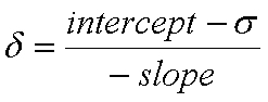
The above equation produces scaled chemical shift values (δ relative to TMS) from the computed isotropic values (σ) and the slope and intercept of the linear regression analysis (Scaling Factors page).
Computed Chemical Shifts - Generating New Scaling Factors
This section covers how to generate scaling factors for a new level of theory (NMR single-point portion) utilizing existing optimized geometries for the test and probe molecule sets.
The Calculation Files page contains Gaussian03G03a input files with optimized coordinates at several levels of theory for the test and probe molecule sets. These are setup to run linked NMR single-point jobs on all structures in the given set. In addition, the catnmrgen, testnmrparse, and probenmrparse Linux scripts are provided to facilitate setting up the jobs for the specific level of theory needed and to extract the information once the jobs have completed. Finally, the template.xls spreadsheet file is provided to easily process the extracted data and produce the scaling factors associated with the new level of theory. Disclaimer: We have found these files to be useful for running and processing NMR jobs on our own system, but we cannot guarantee that all will function exactly as intended on other systems. We also do not intend to endorse any specific commercial software program.
Suggested steps:
- Run catnmrgen on the test and probe set input files (these file names are required arguments for the script). You will be prompted for an output file name and the route section command for your desired NMR single-point method. The script produces ready-to-run G03G03a input files, with one caveat. The caveat is that the script is only able to write the route section for each molecule. Any lines that need to be read in from the bottom (e.g., solvent specification information) must be added to each structure manually (this can be accomplished fairly quickly by copying and pasting). In any case, be sure to inspect the final file to ensure that it has been generated correctly.
- Run the two jobs on your system and ensure that all linked steps complete without error.
- Run the testnmrparse and probenmrparse scripts on the output files from step 2 above. You will be prompted to answer whether or not the NMR method involved the CSGT (as opposed to GIAO, which is default) and MP2 methods; these affect the structure of the output file and thus how the data is to be parsed out. The script will produce three output files - one contains all the crude NMR data while the other two contain 1H and 13C data pre-formatted for the next step.
- Utilize the template.xls spreadsheet by pasting in data from the 1H and 13C data files produced above for both the test and probe sets. The template.xls and nmrparse scripts have been carefully designed to work with each other. The user should only need to copy and paste data into the yellow column of cells (pasting values only - e.g. {edit - paste special - values} is recommended to preserve the formatting) in order to fully populate each tab in the spreadsheet with the relevant data, graph, scaling factors, and performance data.
- Because the test set of molecules contains many chlorine atoms which can adversely affect the 13C scaling factors through relativistic effects,Tan12a we recommend making a duplicate of the Test-13C tab in the spreadsheet and in this new tab, deleting all data for carbon atoms attached directly to chlorine. Specifically, we suggest deleting data in columns C-K for the following rows: 6, 7, 10, 12, 19, 23-25, 38, 45, 50, 54, 70, 76, 103, 113, 158, 159, and 323. Doing so will produce scaling factors that are free from specific error due to relativistic effects.
Computed Chemical Shifts - Re-optimizing Test and Probe Set Geometries
This section covers how to re-optimize the test and probe set geometries in order to generate scaling factors (via the steps above) for new levels of theory at the geometry optimization stage.
The Calculation Files page contains Gaussian03G03a input files with starting coordinates for the test and probe molecule sets. These are setup to run linked geometry optimization jobs on all structures in the given set. In addition, the concatfilemodifier and geomextract Linux scripts are provided to facilitate setting up the jobs for the specific level of theory needed and to prepare an input file suitable for conducting the steps outlined above for generating new scaling factors. Again, we have found these files to be useful for running jobs on our own system, but we cannot guarantee that all will function exactly as intended on other systems.
Suggested steps:
- Run the concatfilemodifier script on the generic input files for the test and probe sets (these file names are required arguments for the script). You will be prompted to specify the amount of memory to use (in MB, don't include the units in your response), the desired route section for the geometry optimization method, and a file name. We strongly recommend including a freq specification in the route section in order to run a frequency analysis on each optimized structure (see step 4 below). The script produces ready-to-run G03G03a input files; be sure to inspect these to make sure they have been generated correctly.
- Run the two jobs on your system and ensure that all linked steps complete without error.
- Run the geomextract script on the resulting output files to generate new input files suitable for NMR single-point calculations as described above.
- Unfortunately, we have found in our experience that it is likely that several molecules in each set will come back with imaginary frequencies after being optimized with a new method. We feel that it is important that all molecules be free of imaginary frequencies before moving on at this point. We therefore suggest searching for the occurrence of "negative" in the resulting output files, and manually re-optimizing any structures that do possess imaginary frequencies. Our preferred method involves extracting the offending coordinates into separate output files, opening them in GaussView, and perturbing the structure along the imaginary frequency coordinate before re-optimizing each structure. Once re-optimized and free of imaginary frequencies, the coordinates can be re-inserted into the input file generated in step 3 above. This whole process is tedious at best, but is nonetheless important for generating meaningful data in the end.
1H-1H Coupling Constants and Computed Chemical Shifts
For 1H-1H coupling constants, an alternative to the procedure listed on the Recommendations Page is to restrict the enhancement of the basis set to only H atoms. This is accomplished by the procedure below.
- Optimize the geometry with B3LYP/6-31G(d).
- Run an NMR single-point calculation in
GAUSSIANG03a,G09a as specified below.
#n B3LYP/gen nmr=(FCOnly,ReadAtoms) int=nobasistransform
The enhanced basis set for H is then included directly in the input file, while the 6-31G(d,p) basis set is specified for all other atoms (this must be done individually for each atom type).
At the end of the molecule specification (separated by a blank line) read in: atoms=H
A sample input file for chloroethane can be viewed by clicking here. - From the resulting log file, extract the desired Fermi contact J values, and scale them by a factor of 0.9155
We have also provided a set of scripts to aid in the calculation of complete proton NMR spectra (chemical shifts and coupling constants) using our most recommended method, which consists of:
- a B3LYP/6-31G(d) gas-phase geometry optimization followed by
- the calculation of magnetic shieldings at WP04/cc-pVDZ level using the NMR=GIAO method and SCRF(solvent=chloroform);
- the computation of scaled chemical shift values δ by the equation:
δ = (31.844 – m) / 1.0205,
where m is the calculated isotropic magnetic shielding; - the calculation of 1H-1H Fermi contact terms at the B3LYP/6-31G(d,p)u+1s[H] level;
- the computation of scaled proton-proton coupling constants through multiplication of the calculated Fermi contact terms by 0.9155.
The scripts may be invoked with an argument that corresponds to a filename which will be abbreviated below as “fff”. If no argument is given, the user is prompted for the filename. Filenames can be given with or without an extension; if no extension is given, a default will be assumed which depends on the case (see below). Scripts 4 and 5 require additional input for which the user is prompted.
- {get_geom fff} extracts the optimized geometry from a B3LYP/6-31 G(d) optimization; input is a Gaussian fff.out (or fff.log) file, the output is a fff.xyz file.
- {mk_input_file fff} generates a Gaussian input file (fff_nmr.inp), using the geometry in the “fff.xyz” file generated by get_geom.
- {extract_spectrum fff_nmr} extracts the 1H chemical shifts and the 1H-1H coupling constants from a Gaussian output file_nmr (fff_nmr.out/log), performs the empirical scaling, and tabulates chemical shifts and coupling constants in a file fff_nmr.txt.
- {average_spectrum fff_nmr} performs averaging between degenerate conformations; input is an fff_nmr.txt file, output an fff_nmr_avg.txt file.
- {average_molecules} performs averaging between non-degenerate conformations; input is a series of fff_nmr.txt (or fff_nmr_avg.txt) files. The output filename is specified by the user.
To carry out the calculation of an entire proton NMR spectrum, the procedure is as described below. Note that, to invoke a script under Linux, it must be preceded by "./" if it resides in the same directory, or by the pathname if it resides in a directory that is different from the one from where it is invoked. Filenames can be specified without extension if the extension corresponds to the default (.out, .log, .xyz, .txt, depending on the case, see below), else the extension must be specified.
- Run a gas-phase B3LYP/6-31G(d) optimization, the output of which appears in a file fff.out or fff.log (where "fff" stands for the filename).
- Invoke get_geom as follows: get_geom fff. A file fff.xyz containing the cartesians will be created.
- Invoke mk_input_file as follows: mk_input_file fff. A file fff_nmr.inp containing the input file for the Gaussian NMR calculation will be created.
- Run the Gaussian calculation with fff_nmr.inp as input.
- Invoke extract_spectrum as follows: extract_spectrum fff_nmr The script will ask the user whether the Gaussian output file contains the default recommended procedures, or something else. In the former case, scaling is performed automatically; in the latter case, the script requests scaling factors from the user. If mk_input_file is used to generate the NMR calculation input file, the output file will indeed correspond to the default method, and the user can reply "y". Chemical shifts and coupling constants for the proton NMR spectrum will appear in a file fff_nmr.txt.
- If the structure contains protons that become equivalent through averaging of degenerate conformations (e.g., the hydrogen atoms of a methyl group), invoke average_spectrum as follows: average_spectrum fff_nmr.txt The script then prompts the user for groups of hydrogen atoms that become equivalent by averaging on the timescale of the experiment. The script also asks the user whether or not to set mutual couplings within an averaged set to zero. Since these couplings are not observable in a typical spectrum, setting them to zero can sometimes simplify spectral simulation calculations without loss of accuracy. The output goes into a file fff_nmr_avg.txt.
- If the molecule has multiple non-degenerate conformations that need to be averaged, invoke the averaging script by typing simply average_molecules. The script then prompts the user for a list of fff_nmr.txt files and corresponding relative free energies; relative free energies should be provided on whatever basis desired by the user. The script also prompts for a temperature.